Atomistic simulations are often restricted by timescale limitations when systems become trapped in metastable energy basins. The transitions between these metastable states are rare events and they dictate the long-term evolution of the system. We present an importance sampling framework to accelerate the time scale of Langevin dynamics simulations. The framework uses a neural network parameterized importance function to bias the dynamics, enhancing the efficiency of rare-transition sampling while preserving relative probabilities between transition paths. We provide a rigorous mathematical formulation to recover the original transition rates between metastable states from the biased dynamics, and use a branching random walk algorithm to control the statistical variance of the estimated rates. We validate the framework on a two-dimensional problem, as well as the system of 7 Lennard-Jones discs as a benchmark atomistic model. The framework provides a scalable foundation for accelerating the simulation of rare events in atomistic systems.
1. Introduction
Atomistic simulations[1]–[3] are powerful tools to elucidate the fundamental mechanisms of physical processes at the molecular scale. However, their applicability is fundamentally constrained by the time scales accessible to brute-force simulation. This limitation stems from the fact that atomistic systems typically remain confined in energy basins, corresponding to metastable states, for long durations. Escaping to a neighboring basin occurs very rarely, yet it is precisely these rare events that determine the long-term evolution of the system. Using brute-force simulation to predict long-term evolution can therefore be prohibitively expensive. This is known as the rare event problem or the timescale problem[4]–[6].
Various computational methods have been developed to address it. Steered molecular dynamics (SMD)[7], metadynamics (MTD)[8]–[11], and hyperdynamics (HD)[12],[13] introduce external biasing potentials to accelerate transitions. Trajectory-based methods such as forward flux sampling (FFS)[14] and the weighted ensemble (WE) method[15],[16] decompose the configuration space into interfaces or bins and sample short trajectories between them. Transition path theory[17]–[26] establishes a mathematical framework to characterize the statistical ensemble of reactive trajectories. Importance sampling[27]–[30] constitutes another fundamental approach for efficiently sampling reaction pathways and quantifying the kinetics of rare events. This paper focuses on applying importance sampling to Langevin dynamics simulations to extend their timescales.
The proposed framework addresses two objectives. First, it enhances the efficiency of sampling rare transition paths while rigorously preserving the relative probabilities of competing transition channels. Second, it yields an unbiased estimator for the original transition rates by reweighting the ensemble of transition paths generated by the accelerated dynamics. These goals are achieved by modifying the system kinetics via an importance function that biases the transition probability kernels to preferentially sample successful transition paths. The normalization condition of this modified kernel imposes a unique condition that defines the optimal importance function.
Applying this framework to high-dimensional systems presents challenges. Obtaining the optimal importance function is generally intractable, as it requires solving a high-dimensional partial differential equation over a complex energy landscape. Moreover, the accuracy of the transition rate estimator is highly sensitive to the quality of this importance function; even minor approximation errors can induce large fluctuations in the estimated rates and alter the relative probability of competing pathways. To obtain a suitable importance function in high dimensions we parameterize it with a neural network and optimize it via adaptive training. To tolerate the unavoidable approximation error, we construct an unbiased estimator for the transition rate even when the importance function is not strictly optimal, by assigning statistical weights to the sampled transition paths. Finally, to increase efficiency and reduce variance, we use a branching random walk (BRW) algorithm[31] to regulate the weights of the sampled paths.
2. Problem Statement
Consider a system specified by a position vector $\mathbf{x}$ that exists in a domain $\Omega$, on which a potential energy $U(\mathbf{x})$ is defined, as shown in Figure 1. The energy landscape is characterized by two deep basins corresponding to two metastable states, $\Omega_{\rm A}$ and $\Omega_{\rm B}$. Each metastable state is the collection of all microscopic states that lead to the same local energy minimum under a steepest-descent trajectory of $U(\mathbf{x})$. The time evolution of the system at temperature $T$ is governed by the overdamped Langevin dynamics[32],
where $\beta = 1/(k_{\rm B} T)$, $k_{\rm B}$ is the Boltzmann constant, $\gamma$ is the friction coefficient, and $\mathbf{W}(t)$ is the standard Wiener process. Although Fig. 1 depicts a two-dimensional domain, the target is systems of arbitrary dimension $d$, in which both $\mathbf{x}$ and $\mathbf{W}$ are $d$-dimensional vectors. The stochastic process described by Eq. (1) has a stationary distribution given by the Gibbs–Boltzmann distribution[33],
Because $\rho_{\rm eq}(\mathbf{x})$ is heavily concentrated around the local minima of the basins, a system initialized in $\Omega_{\rm A}$ tends to stay within $\Omega_{\rm A}$ for a long time before making a rare transition into $\Omega_{\rm B}$.
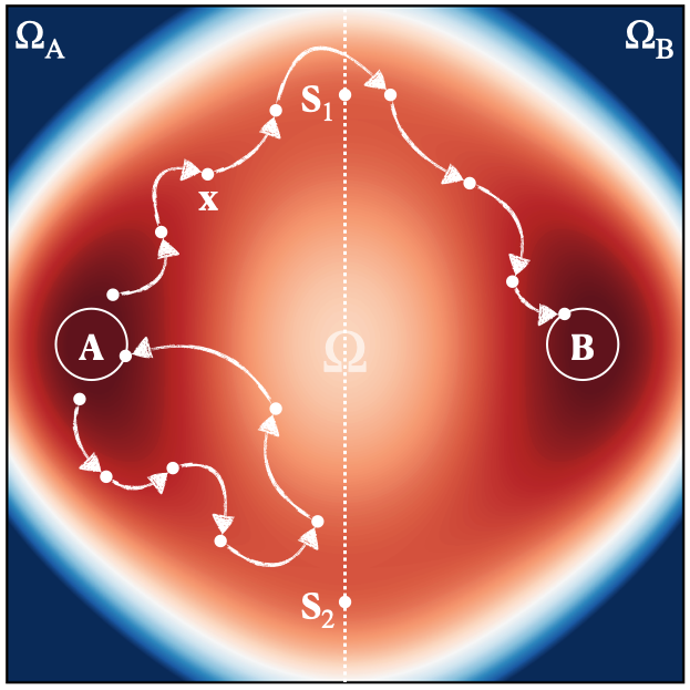
We define two small regions A and B around the local minima of $\Omega_{\rm A}$ and $\Omega_{\rm B}$. A trajectory initialized in $\Omega_{\rm A}$ visits region A repeatedly, for a long time, before it ever visits region B. This lets us break a long-time trajectory into many short trajectories (called paths), as illustrated in Figure 2. Paths that leave region A and return to A before visiting B are called failure paths; those that leave A and visit B before returning are called success paths. Our first objective is to enhance the probability of sampling success paths uniformly, so that the relative probability of escaping $\Omega_{\rm A}$ via different channels (e.g. near $S_1$ or $S_2$) remains unchanged. The second is to know exactly by how much this probability has been enhanced, so that we can recover the escape rate of the original system.
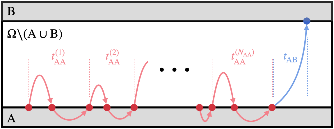
The transition rate $r_{\rm AB}$ from $\Omega_{\rm A}$ to $\Omega_{\rm B}$ is obtained from the mean first passage time $t_{\rm FPT}$ from region A to region B,
Since the system repeatedly visits region A before reaching B, the mean first passage time takes the form
where $\langle N_{\rm AA}\rangle$ is the average number of failure paths sampled before a success path, $\langle t_{\rm AA}\rangle$ is the mean time interval between successive escapes from A, and $\langle t_{\rm AB}\rangle$ is the average time of a success path. The average number of failed attempts follows from a geometric sum,
where $P_{\rm AB}$ is the probability of sampling a success path from A (the success probability). When the system exhibits a rare-event problem, $P_{\rm AB} \ll 1$, and
This yields the transition rate
The inverse of $\langle t_{\rm AA}\rangle$ is the flux $J_{\rm A}$ out of A, known as the Hill relation[34]–[37]. The mean time between escapes can be estimated cheaply from unbiased equilibrium simulations near A (Section 3.6). Since $P_{\rm AB}$ is vanishingly small, computing it by brute force is very inefficient. Our goal is to modify the kinetics so that $P_{\rm AB}$ is enhanced while the relative probability of different success paths remains unchanged.
3. Methods
3.1 Langevin Dynamics and Path Sampling
The overdamped Langevin dynamics of Eq. (1) is simulated with a time step $\Delta t$ using the Euler–Maruyama scheme[38],
where $\boldsymbol{\xi}$ is a vector of independent standard Gaussian random variables. A path is a sequence of microscopic states visited along the trajectory,
A path is initiated (at $\mathbf{x}_1$) whenever the trajectory leaves region A, and terminated whenever it enters region A or region B, i.e. $\mathbf{x}_N \in \mathrm{A}\cup\mathrm{B}$. Paths terminating in A ($\Gamma_{\rm AA}$) are failure paths; those terminating in B ($\Gamma_{\rm AB}$) are success paths. To coarse-grain time, successive stored states are separated by a period $\tau = k\Delta t$ with $k$ a positive integer, except that the final step may be shorter if the system enters A or B first.
3.2 Importance Sampling of Transition Paths
Let $\mathcal{K}_\tau(\mathbf{y}\,|\,\mathbf{x})$ be the probability density kernel of visiting $\mathbf{y}$ as the next microscopic state on a path given the current state $\mathbf{x}$, where the time separation equals $\tau$ or the first passage time $\tau_{\rm A\cup B}$ to region A or B, whichever is smaller,
with $\delta(\cdot)$ the $d$-dimensional Dirac delta and $\wedge$ the minimum. The probability density of sampling a success path is
where $\rho_{\rm A}(\mathbf{x}_1)$ is the density of the initial state at the moment of exiting A (Section 3.6). The success probability is the integral over all success paths,
To alter the kinetics we modify the kernel with an importance function $I(\mathbf{x})$[28],[29],
The modified kernel must satisfy the normalization condition $\int_{\mathbf{y}\in\Omega} d\mathbf{y}\, \mathcal{K}'_\tau(\mathbf{y}\,|\,\mathbf{x}) = 1$ (Eq. 15). We define the importance function that satisfies this everywhere as the optimal importance function $I_{\rm opt}(\mathbf{x})$. When $I(\mathbf{x}) \neq I_{\rm opt}(\mathbf{x})$, the kernel must be renormalized by a factor $Z_\tau(\mathbf{x})$,
The biased path density $p'(\Gamma_{\rm AB}) = \rho_{\rm A}(\mathbf{x}_1)\prod_{i=1}^{N-1}\mathcal{K}'_\tau(\mathbf{x}_{i+1}\,|\,\mathbf{x}_i)$ (Eq. 18) can be rewritten by inserting Eq. (16),
If the importance function is optimal, all normalization factors equal unity and this simplifies to
The enhancement factor $I_{\rm opt}(\mathbf{x}_N)/I_{\rm opt}(\mathbf{x}_1)$ is independent of the intermediate positions and is explicitly known, so the unbiased path density can be reconstructed from the biased dynamics. In practice $I_{\rm opt}(\mathbf{x})$ is generally unknown; the normalization condition provides an optimality target,
Setting $I(\mathbf{x}) = 0$ for $\mathbf{x}\in\mathrm{A}$ and $I(\mathbf{x}) = 1$ for $\mathbf{x}\in\mathrm{B}$, the optimal importance function quantifies the probability of reaching B before returning to A, i.e. the committor function[17]. The evolution under $\mathcal{K}'_\tau$ is equivalent to overdamped Langevin dynamics with an added bias potential,
This bias potential is the “optimal controller”[39]–[41], derived from the Doob $h$-transform[42] or the Girsanov theorem[43]–[45].
3.3 Success Probability Estimation
Defining a reward function $R(\Gamma) = 1$ if $\Gamma \in \{\Gamma_{\rm AB}\}$ and $0$ otherwise (Eq. 24), the success probability is the expectation of $R$ over all paths sampled with $\mathcal{K}_\tau$, $P_{\rm AB} = \mathbb{E}_\Gamma[R(\Gamma)]$ (Eqs. 25–26). This is intractable under rare-event conditions because almost all sampled paths have zero reward. Sampling instead under the biased kernel $\mathcal{K}'_\tau$ and reweighting with Eq. (19) gives
Defining the path weight
the success probability becomes an expectation over paths sampled with $\mathcal{K}'_\tau$,
The advantage is that $\mathcal{K}'_\tau$ preferentially samples successful paths with non-zero reward. In the ideal limit $I(\mathbf{x}) = I_{\rm opt}(\mathbf{x})$ this reduces to the “reactive probability”[37],[46],
Replacing $I_{\rm opt}$ by its approximation $I$ in Eq. (31) would introduce uncontrolled error, as demonstrated in Section 4. The full weighted average in Eq. (30) is required for an unbiased estimate.
3.4 Branching Random Walk
Although Eq. (30) is unbiased, its statistical convergence depends on the quality of $I(\mathbf{x})$: the closer $I$ is to $I_{\rm opt}$, the smaller the variance of the path weights $W(\Gamma)$. Even a small deviation can produce large weight fluctuations. We combine a branching random walk (BRW)[31] with the biased path sampling. Each walker starts with state $\mathbf{x}_1 \sim \rho_{\rm A}$ and unit weight; at each step its weight is multiplied by the current normalization factor. If the weight stays within a predefined range $[W_{\min}, W_{\max}]$ the walker continues; otherwise it branches into $\mathcal{R}(W)$ walkers using stochastic rounding,
with branched walkers reset to unit weight to preserve the total weight. There are three cases: $\mathcal{R}(W) = 0$ terminates the walker; $\mathcal{R}(W) = 1$ continues it with weight reset to unity; $\mathcal{R}(W) > 1$ branches it into multiple unit-weight walkers. Each “success” walker then receives a reward equal to its weight times $I(\mathbf{x}_1)/I(\mathbf{x}_N)$, and the success probability is estimated by averaging rewards following Eq. (29). By regulating the walker weights, the BRW controls the variance of the estimator.
3.5 Optimization of Importance Function
In high dimensions the configuration volume grows exponentially, so we approximate the importance function with a neural network $I(\mathbf{x};\theta)$, where $\theta$ are the trainable parameters[37],[50],[51]. We optimize it by minimizing the loss[37],[52]
where $g(\mathbf{x}) > 0$ is a distribution function. The loss reaches its global minimum of $0$ when $I(\mathbf{x};\theta) = I_{\rm opt}(\mathbf{x})$. Because evaluating the loss over all of $\Omega$ is intractable, we evaluate it only on microscopic states $\mathbf{x}$ sampled by the importance sampling procedure itself, giving an adaptive training scheme (Algorithm 1).
- Initialize neural network parameters $\theta$; initialize replay library $\mathcal{M} \leftarrow \emptyset$.
- Initialize $n$ walkers near the boundary of A according to $\rho_{\rm A}(\mathbf{x})$.
- while not converged do:
1. Sampling stage
- Propagate walkers using the biased kernel $\mathcal{K}_\tau$ driven by the current $I(\mathbf{x};\theta)$; collect newly visited states $\mathcal{S}_{\rm new}$.
- If a walker reaches region B (success path), append its states to the library $\mathcal{M}$.
2. Training stage- Sample a new batch $\mathcal{B}_{\rm new}$ from $\mathcal{S}_{\rm new}$ and a historical batch $\mathcal{B}_{\rm lib}$ from $\mathcal{M}$.
- Update $\theta \leftarrow \theta - \eta\,\nabla_\theta \sum_{\mathbf{x}\in\mathcal{B}} \mathcal{L}(\mathbf{x},\theta)$ over $\mathcal{B} = \mathcal{B}_{\rm new}\cup\mathcal{B}_{\rm lib}$.
3.6 Sampling Initial States of Paths
Escaping region A is not a rare event, so the mean time $\langle t_{\rm AA}\rangle$ between successive escapes can be computed from a standard unbiased Langevin simulation initialized in A. Recording the sequence of escape times $\{t_1, t_2, \ldots, t_L\}$ (Eq. 35), the mean interval is
3.7 Computing the Normalization Factor
Computing $Z_\tau(\mathbf{x})$ by quadrature is infeasible in high dimensions, but an unbiased Monte Carlo estimate is available. We generate $M$ independent trajectories initiated at $\mathbf{x}$, each propagated under $\mathcal{K}_\tau$ for $\tau \wedge \tau_{\rm A\cup B}$, record their terminal positions $\{\mathbf{y}_i\}_{i=1}^{M}$, and evaluate
This estimator converges to $Z_\tau(\mathbf{x})$ as $M$ increases. In this work we choose $M = 100$.
3.8 Biased Transition Path Sampling
We reuse the same ensemble of $M$ trajectories from Section 3.7 via sequential importance resampling[57]–[59]. Given terminal positions $\{\mathbf{y}_i\}$ and their importance values $I(\mathbf{y}_i)$, the next state of the importance-sampled path is selected from the ensemble with probability
This avoids computing any gradient of the importance function.
3.9 Reverse Path Sampling
For the reverse process ($\Omega_{\rm B}\to\Omega_{\rm A}$), the optimal biased kernel is simply
because if $I_{\rm opt}$ is optimal for A$\to$B, then $1 - I_{\rm opt}$ is optimal for B$\to$A. The numerical procedure is unchanged apart from replacing $I$ by $1-I$ in Eqs. (37)–(38). Training is modified accordingly by initiating trajectories near the boundaries of both A and B simultaneously, so a single network learns to sample both forward and backward transitions.
4. Results
We validate the framework on a two-dimensional system and the Lennard-Jones 7 (LJ7) benchmark, demonstrating its robustness and scalability.
4.1 Two-Dimensional Potential with Two Reaction Channels
The first benchmark is a two-dimensional potential with two distinct reaction channels[25],[28],[29],[56]. The potential energy (in eV) is
where $\mathbf{x} = [x_1, x_2]^{\top}$ (in nm). The system has minima at $\mathbf{x}_{\rm A} = [-1.1, 0]^{\top}$ nm and $\mathbf{x}_{\rm B} = [1.1, 0]^{\top}$ nm, and saddle points at $\mathbf{x}_{S_1} = [0, 1]^{\top}$ nm and $\mathbf{x}_{S_2} = [0, -1]^{\top}$ nm. The energy barriers are 1.02 eV at $S_1$ and 0.98 eV at $S_2$. Regions A and B are circles of radius $0.1$ nm centered at $\mathbf{x}_{\rm A}$ and $\mathbf{x}_{\rm B}$. Simulations use friction $\gamma = 1$ eV nm$^{-2}$ fs and time step $\Delta t = 10^{-2}$ fs.
The importance function is the logistic sigmoid of a scalar potential $h(\mathbf{x};\theta)$,
with fixed Gaussian parameters $A = 3$, $(a_1, a_2) = (1, 1)$, $(c_1, c_2) = (-1.1, 0)$. The MLP has two hidden layers of 50 neurons each with $\tanh$ activations. A single walker is initialized at $T = 500$ K and training proceeds for 1,000 iterations with the ADAM optimizer[60] at learning rate $5\times10^{-3}$; the exact optimal importance function used for comparison is obtained by the finite element method (FEM)[61].
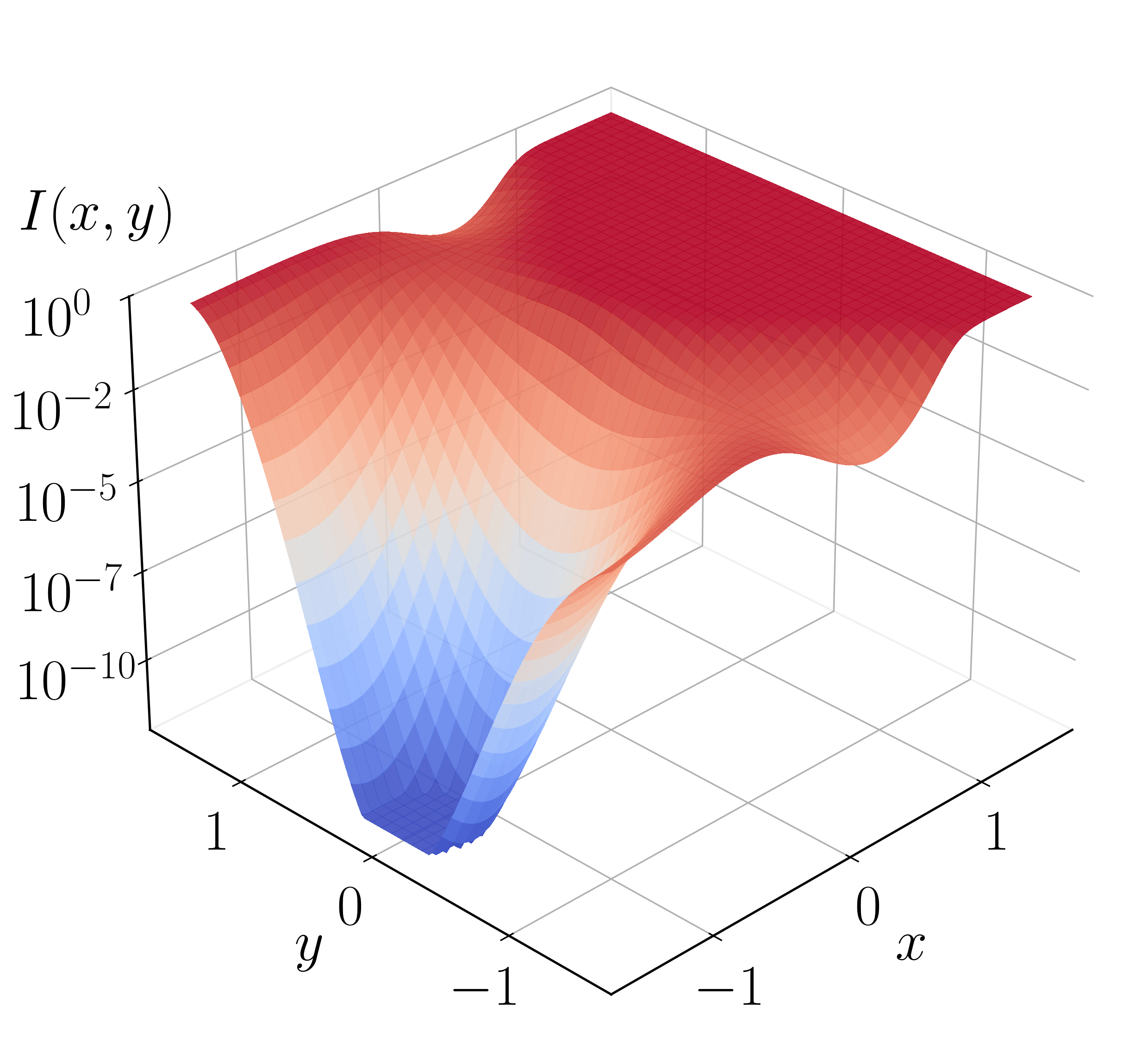
The trained importance function accelerates the transition at $T = 500$ K, sampling paths with the BRW algorithm over 1,000 independent trials of 1,000 paths each and branching weight thresholds $[1.0, 2.0]$. The estimated success probability is $P_{\rm AB} = (9.0067 \pm 0.0558)\times 10^{-13}$. Direct evaluation from Eq. (31), assuming the network is optimal, gives a significantly biased $P_{\rm AB}^{\rm NS} = 3.2028\times 10^{-13}$ (no sampling). The flux out of A is estimated from $10^5$ escape configurations as $J_{\rm A} = 8.0736$ fs$^{-1}$, yielding the transition rate $r_{\rm AB} = (7.2717 \pm 0.0450)\times 10^{-12}$ fs$^{-1}$, in good agreement with Kramers rate theory[56], $r_{\rm AB}^{\rm Kr} = 7.1755\times 10^{-12}$ fs$^{-1}$. Without path sampling the rate is $r_{\rm AB}^{\rm NS} = 2.5858\times 10^{-12}$ fs$^{-1}$, very different from the correct value. The framework also recovers the fraction of transitions through $S_1$: importance sampling gives $0.2972 \pm 0.0023$, close to the Kramers value $0.2938$, whereas direct counting without reweighting gives an inaccurate $0.4483$ (Table 1).
| Method | $r_{\rm AB}$ |
|---|---|
| Importance Sampling | 7.2717 ± 0.0450 |
| Kramers | 7.1755 |
| No Sampling | 2.5858 |
| Method | $r_{\rm AB}(S_1)/r_{\rm AB}$ |
|---|---|
| Importance Sampling | 0.2972 ± 0.0023 |
| Kramers | 0.2938 |
| No Reweighting | 0.4483 |
Table 1. Results for the 2-dimensional system at 500 K. (a) Transition rates from importance sampling, Kramers rate theory, and no sampling (Eq. 31 assuming $I \approx I_{\rm opt}$). (b) Transition rate fraction through $S_1$ from importance sampling, Kramers theory, and direct counting without reweighting.
Repeating the estimation from $500$ K to $1000$ K, the importance sampling rates and $S_1$ fractions agree with Kramers rate theory across temperatures, whereas estimates without path sampling show significant errors, especially at low temperature.
4.2 Sampling Bidirectional Transitions
Using the reverse-sampling scheme of Section 3.9, a single network boosts both forward ($\Omega_{\rm A}\to\Omega_{\rm B}$) and backward ($\Omega_{\rm B}\to\Omega_{\rm A}$) transitions. Here the importance function is the sigmoid of an MLP with no Gaussian term,
For the 2D system the MLP has two hidden layers of 50 neurons ($\tanh$), trained for 2,000 epochs (ADAM, learning rate $5\times10^{-3}$). Sampling both directions during training yields a more accurate importance function after the same number of epochs than sampling only escapes from $\Omega_{\rm A}$, and it removes the need to select a Gaussian term. As summarized in Table 2, the importance-sampling rates $r_{\rm AB}$ and $r_{\rm BA}$ and their $S_1$ fractions agree closely with Kramers theory in both directions, while direct evaluation without reweighting yields significantly biased rates and incorrect fractions.
| Method | $r_{\rm AB}$ | $r_{\rm BA}$ |
|---|---|---|
| Importance Sampling | 7.2093 ± 0.0472 | 7.3635 ± 0.0528 |
| Kramers | 7.1755 | 7.1755 |
| No Sampling | 21.6420 | 25.3386 |
| Method | $r_{\rm AB}(S_1)/r_{\rm AB}$ | $r_{\rm BA}(S_1)/r_{\rm BA}$ |
|---|---|---|
| Importance Sampling | 0.2963 ± 0.0030 | 0.2866 ± 0.0033 |
| Kramers | 0.2938 | 0.2938 |
| No Reweighting | 0.4602 | 0.4619 |
Table 2. Bidirectional results for the 2-dimensional system at 500 K.
4.3 Lennard–Jones 7 (LJ7) System
The most demanding benchmark is the system of 7 Lennard-Jones discs (LJ7), a 14-degree-of-freedom atomistic model[26],[41],[62]. The soft-core potential is
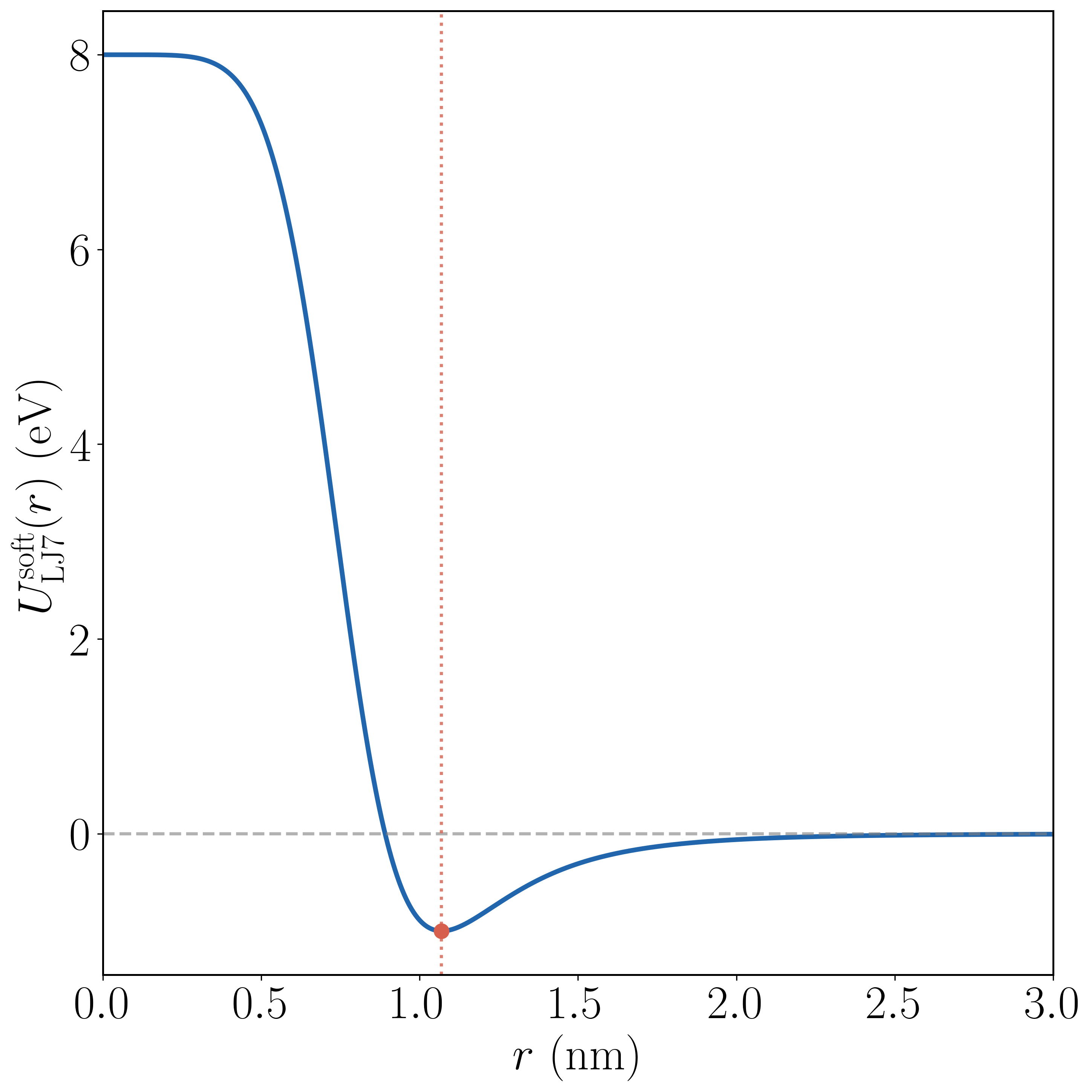
where $r_{ij} = \|\mathbf{x}_i - \mathbf{x}_j\|$, and we choose $\varepsilon = 1.0$ eV, $\alpha = 0.5$, $\varsigma = 1.0$ nm, with time step $\Delta t = 10^{-3}$ fs. The parameter $\alpha > 0$ regularizes the $r_{ij}\to 0$ singularity, replacing the divergent $r_{ij}^{-12}$ repulsion with a large but finite core (Figure 4a), avoiding divergent forces during sampling.
Relaxing all configurations partitions the space into metastable states, each associated with a local energy minimum. After quotienting out continuous (translational and rotational) symmetries, the minima related by discrete symmetries still incur energy barriers and remain distinct. We label collections of such states using a coordination number $c_i$ for each atom,
and the second and third central moments of the coordination numbers[11],[63]–[65],
All local minima group into four collections $C_0, C_1, C_2, C_3$ in $(\mu_2, \mu_3)$ space (Figure 4b).
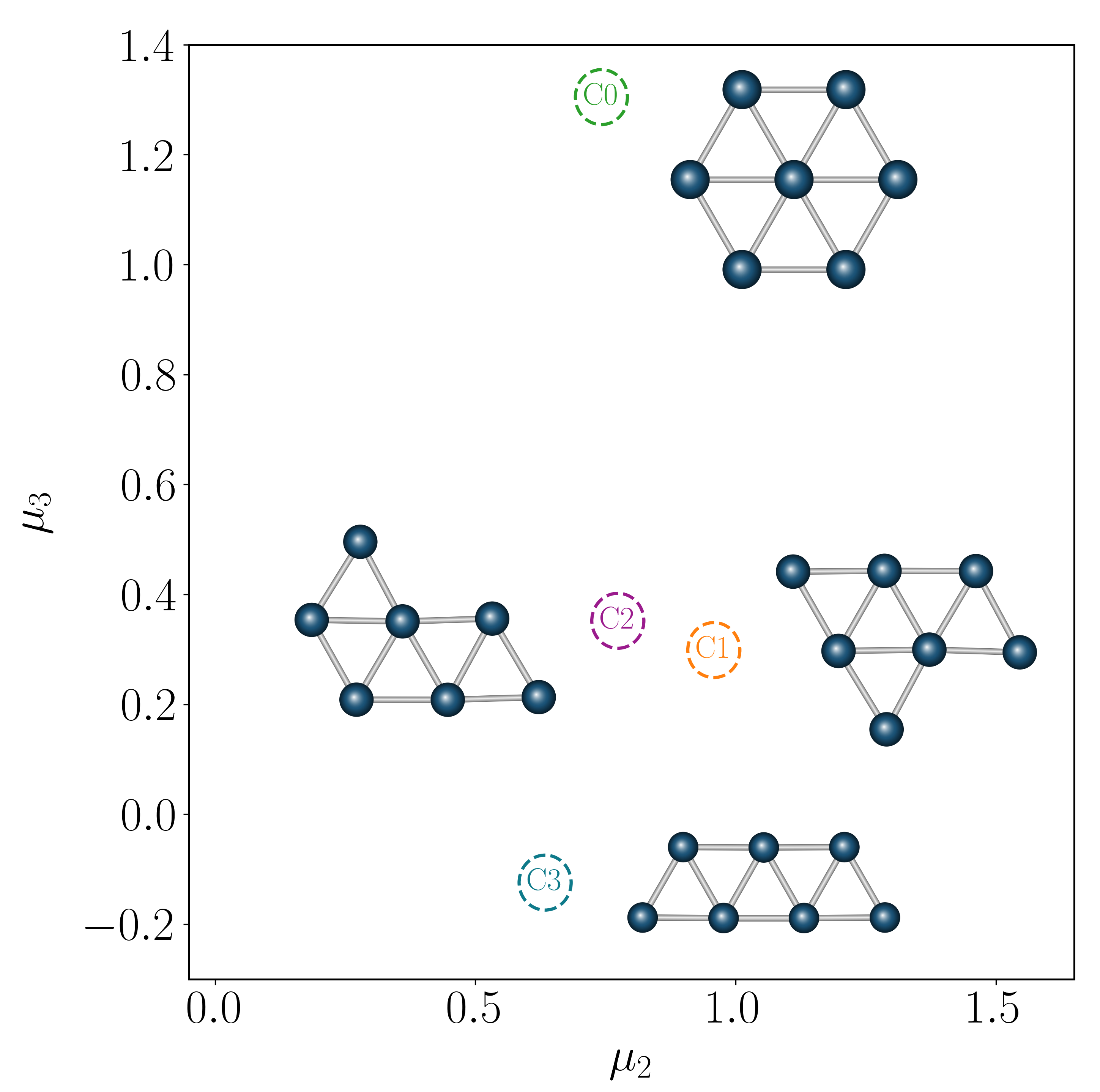
We focus on transitions out of a particular $C_3$ state (region A) into the $C_2$ collection (region B); at low temperatures nearly all transitions out of a $C_3$ state enter a $C_2$ state[24],[26],[66]. There are four distinct transition mechanisms $M_1$–$M_4$, each a coordinated rearrangement of a subset of atoms. Modes $M_1$ and $M_2$ are related by a mirror symmetry of the $C_3$ state, as are $M_3$ and $M_4$. Using the string method[66],[67], the energy barrier heights are 0.49 eV for modes $M_1$ and $M_2$, and 0.52 eV for modes $M_3$ and $M_4$. At $T = 600$ K ($\beta U_{\rm b} \sim 10$) these transitions are rare events.
Region A is defined by a nearest-neighbor distance criterion over the 11 nearest-neighbor pairs $\mathcal{N}_{11}$ at the $C_3$ minimum,
with $\delta_{\rm A} = 0.1\,\varsigma$; region B is a circular region in $(\mu_2, \mu_3)$ space about the $C_2$ minimum,
where $(\mu_2(C_2), \mu_3(C_2)) = (0.7736, 0.3520)$ and $\delta_{\rm B} = 10^{-2}$. Region B encompasses all four transition modes, since the $C_2$ states are permutationally distinct but share the same $(\mu_2, \mu_3)$.
The importance function is a lightweight SchNet-style graph neural network[68] acting on pairwise distances $r_{ij}$, invariant under translations, rotations, and permutations of identical atoms. Distances are expanded in a radial basis,
atom features are updated through $L$ interaction layers with continuous filters,
and a per-atom readout followed by summation and a sigmoid gives the importance function,
We use $n_{\rm f} = 64$ features, $n_{\rm rbf} = 50$ radial basis functions, and $L = 3$ interaction layers ($\approx 6\times 10^4$ parameters). Training targets the $C_3 \to C_2$ transition at $T = 600$ K for 11,000 epochs (ADAM, learning rate $5\times 10^{-4}$); the final model averages checkpoints saved every 200 epochs over the last 1,000 epochs[69]. Along the minimum energy paths[66], the learned importance function increases monotonically from $I \sim 10^{-8}$ near $C_3$ to $I \approx 1$ near $C_2$, reaching $I \approx 0.5$ at the transition state.
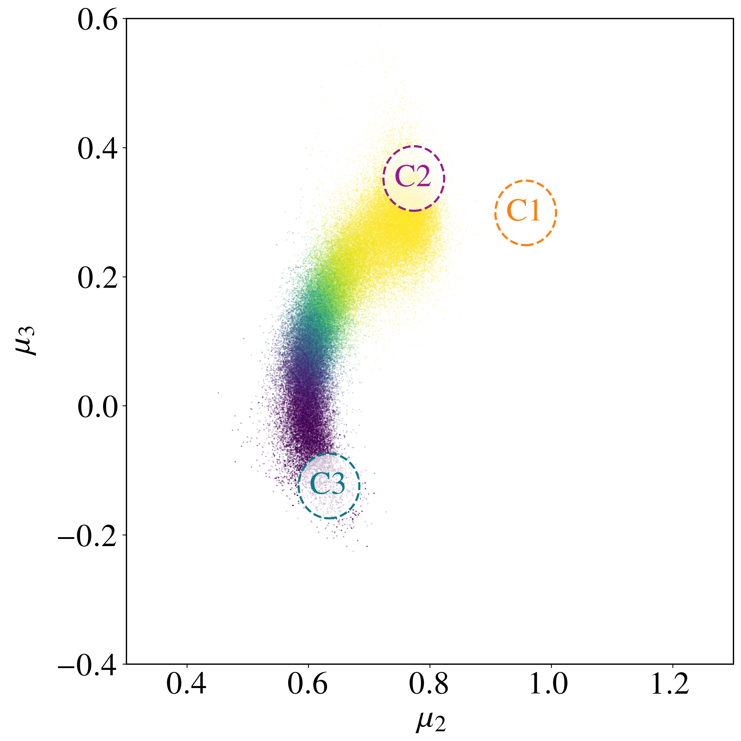
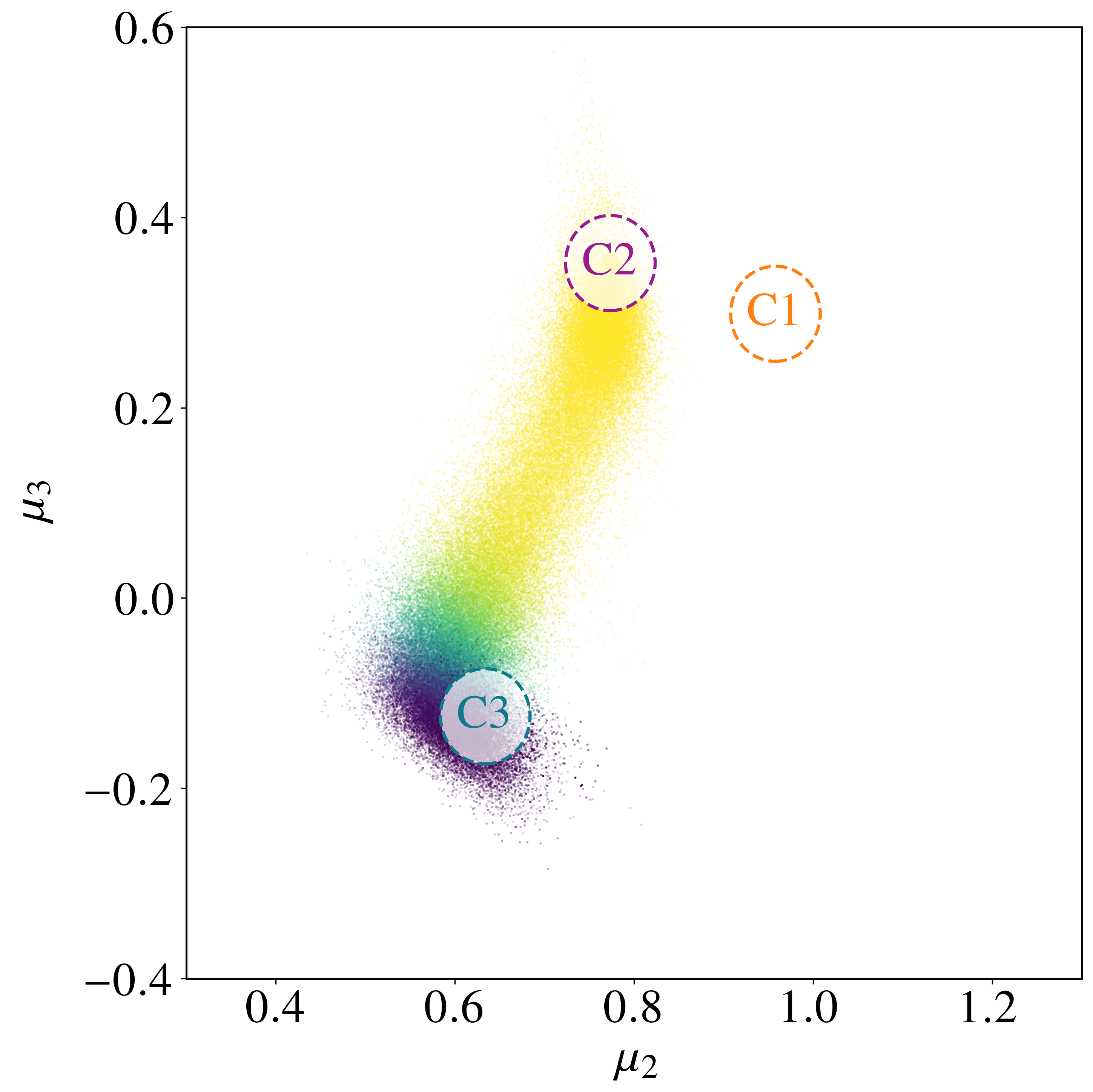
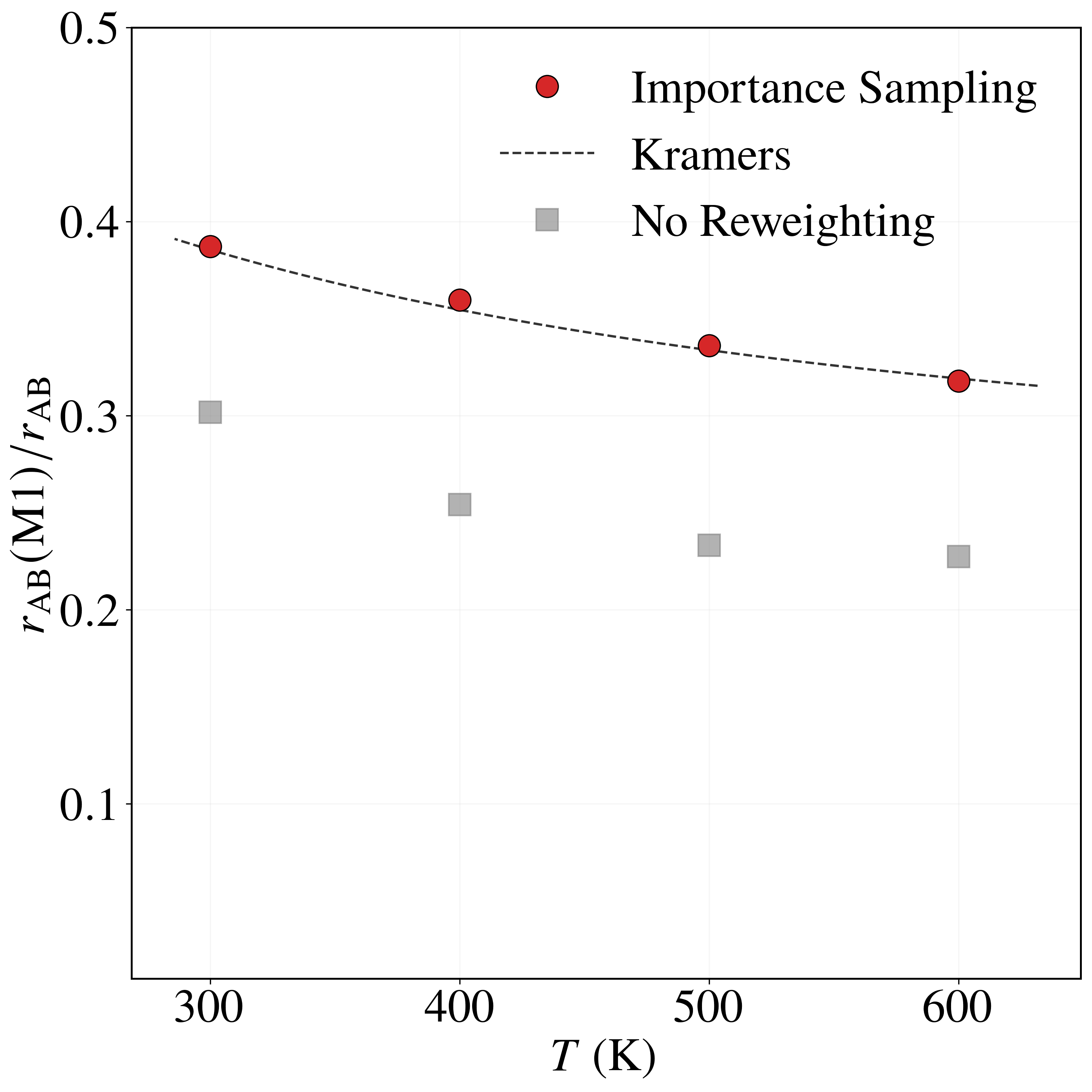
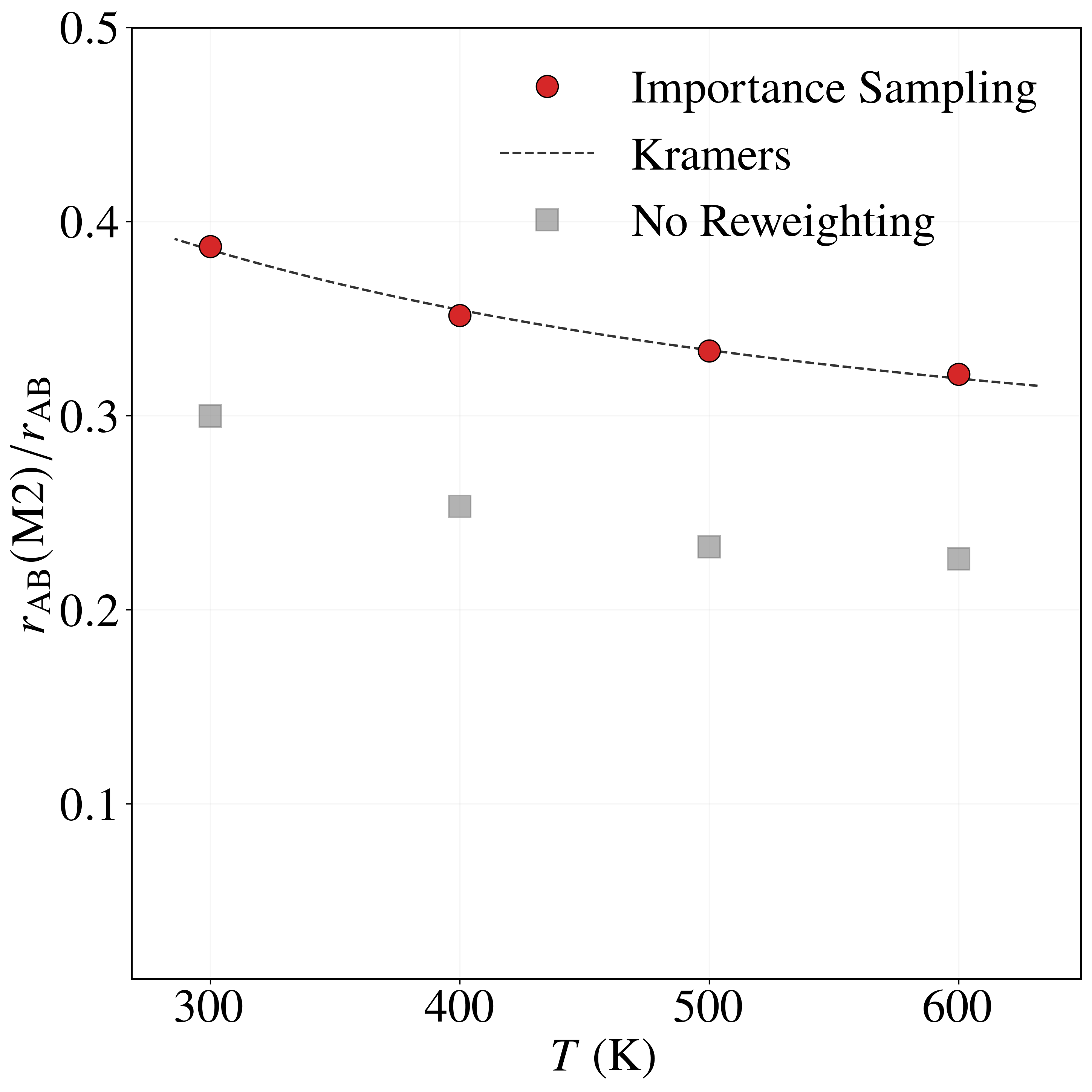
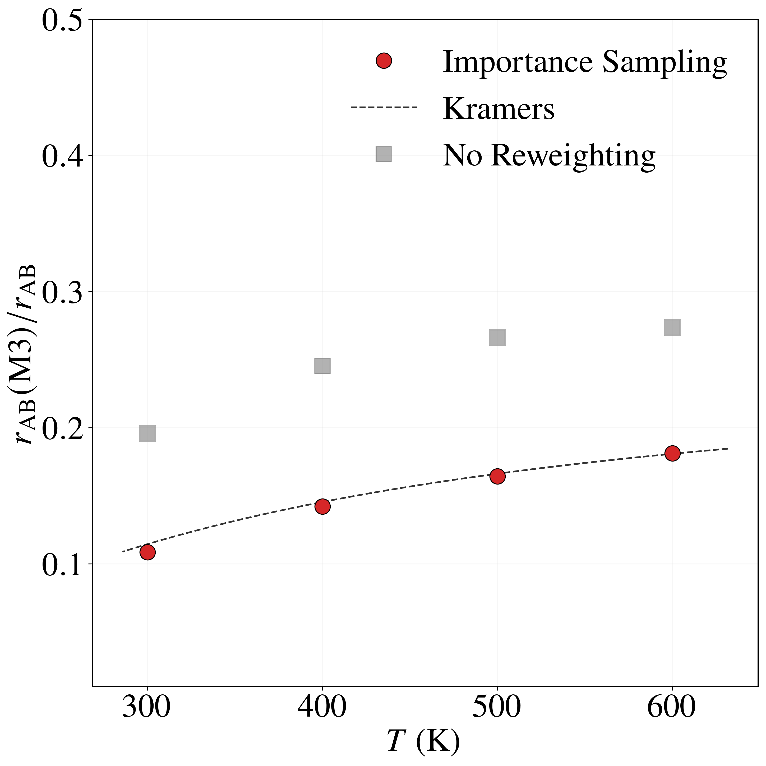
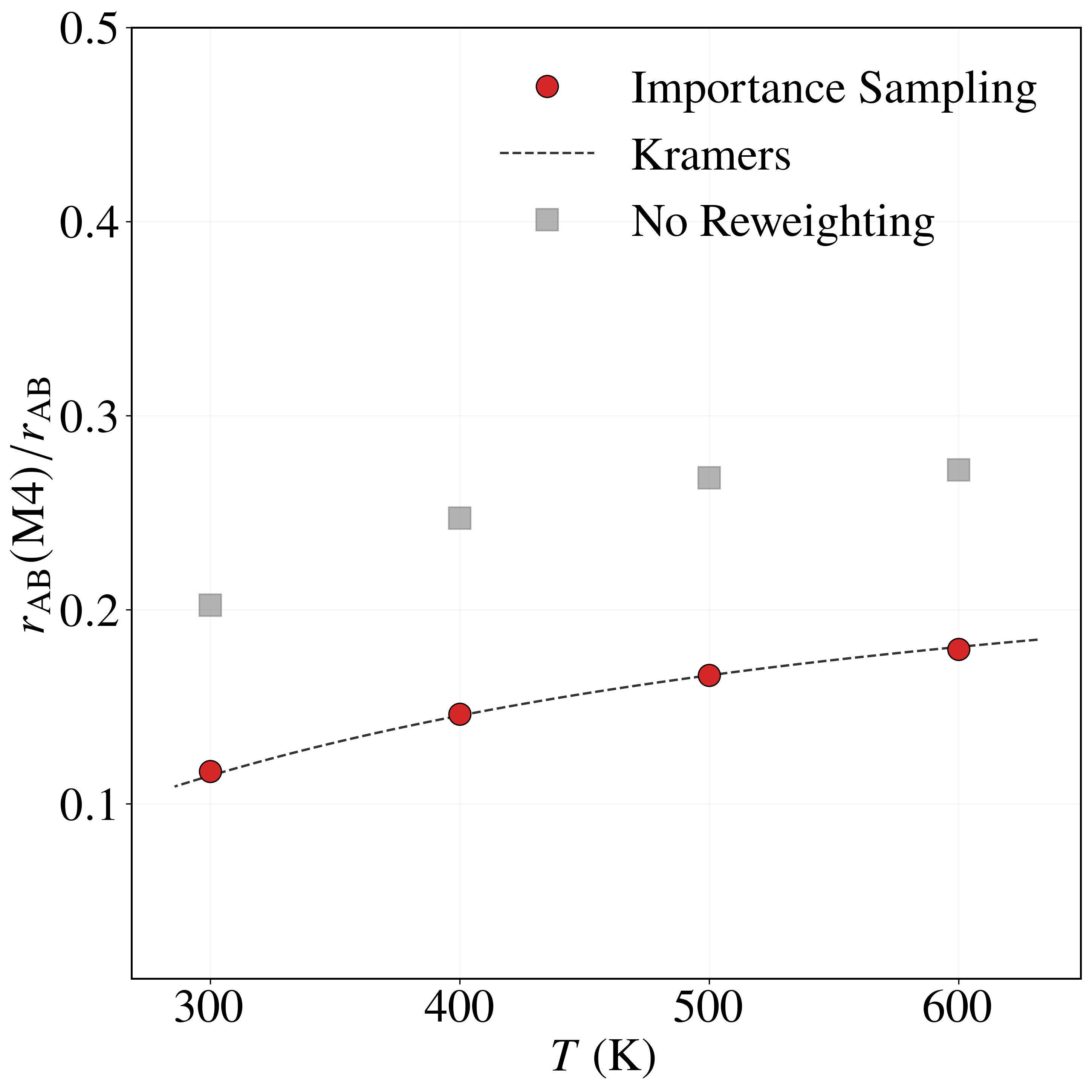
Sampling with the BRW algorithm over 1,000 trials of 1,000 paths each (weights $[1.0, 2.0]$, repeated 10 times with different seeds) gives $P_{\rm AB} = (8.6491 \pm 0.0196)\times 10^{-6}$, versus $P_{\rm AB}^{\rm NS} = (5.2284 \pm 0.0571)\times 10^{-6}$ without path sampling. With flux $J_{\rm A} = (4.9969 \pm 0.0122)\times 10^{1}$ fs$^{-1}$, the rate is $r_{\rm AB} = (4.3215 \pm 0.0098)\times 10^{-4}$ fs$^{-1}$, in excellent agreement with the brute-force value $r_{\rm AB}^{\rm BF} = 4.4110\times 10^{-4}$ fs$^{-1}$. Without path sampling, $r_{\rm AB}^{\rm NS} = (2.6123 \pm 0.0026)\times 10^{-4}$ fs$^{-1}$, an underestimate of about 40%. The framework also resolves the four mechanisms: modes $M_1$ and $M_2$ each carry $\approx 32\%$ of the rate and modes $M_3$ and $M_4$ each $\approx 18\%$, an asymmetry consistent with the higher $0.52$ eV barrier of $M_3, M_4$ versus $0.49$ eV for $M_1, M_2$. The no-reweighting estimate incorrectly predicts a nearly uniform split (Table 3).
| Method | $r_{\rm AB}(M_1)/r_{\rm AB}$ | $r_{\rm AB}(M_2)/r_{\rm AB}$ | $r_{\rm AB}(M_3)/r_{\rm AB}$ | $r_{\rm AB}(M_4)/r_{\rm AB}$ | $r_{\rm AB}$ |
|---|---|---|---|---|---|
| Importance Sampling | 0.3178 | 0.3213 | 0.1811 | 0.1797 | 4.3215 ± 0.0098 |
| Brute Force | 0.3192 | 0.3170 | 0.1838 | 0.1795 | 4.4110 |
| Kramers | 0.3191 | 0.3191 | 0.1809 | 0.1809 | 4.6631 |
| No Reweighting | 0.2273 | 0.2263 | 0.2736 | 0.2721 | 2.6123 ± 0.0747 |
Table 3. Relative transition probabilities $r_{\rm AB}(M_k)/r_{\rm AB}$ through each mechanism and total transition rates $r_{\rm AB}$ (in $10^{-4}$ fs$^{-1}$) for the LJ7 system at 600 K, from importance sampling, brute-force Langevin dynamics, Kramers theory, and no sampling / no reweighting (Eq. 31 assuming $I \approx I_{\rm opt}$).
4.4 Lennard–Jones (LJ7) System Across Temperatures
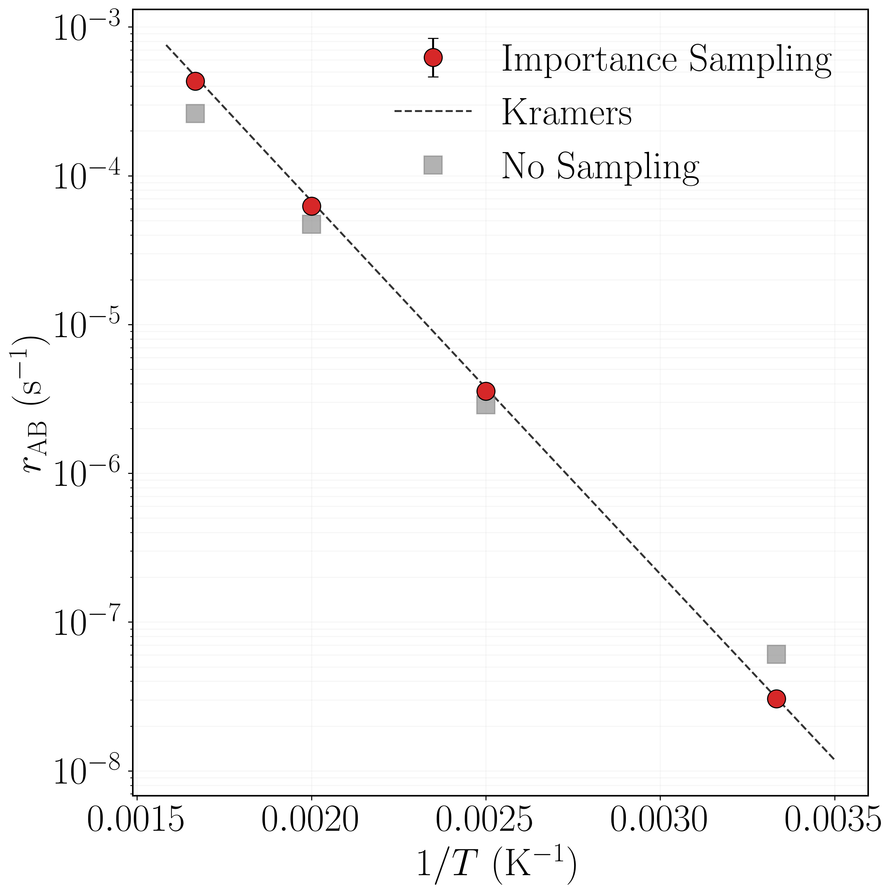
Because the optimal importance function is temperature dependent, the network must in principle be retrained at each temperature. To avoid this cost we use transfer learning[70]: the network trained at $T = 600$ K (Section 4.4) is used as the initial model for fine-tuning at $T = 500, 400, 300$ K. At each temperature, 1,000 trials of 1,000 paths are performed with the BRW algorithm, repeated 10 times. The estimated rates are
in good agreement with the Kramers predictions $r_{\rm AB}^{\rm Kr}(500\,\text{K}) = 6.7588\times 10^{-5}$, $r_{\rm AB}^{\rm Kr}(400\,\text{K}) = 3.7553\times 10^{-6}$, and $r_{\rm AB}^{\rm Kr}(300\,\text{K}) = 3.0898\times 10^{-8}$ fs$^{-1}$ (brute force cannot accumulate sufficient statistics at these low temperatures). Agreement with Kramers theory in fact improves at lower temperatures, where its harmonic approximation becomes more accurate. Without path sampling the estimates $r_{\rm AB}^{\rm NS} = 4.7271\times 10^{-5}$, $2.8839\times 10^{-6}$, and $6.0849\times 10^{-8}$ fs$^{-1}$ deviate systematically; at $300$ K the no-sampling estimate overshoots by nearly a factor of two.
As the temperature decreases from $600$ K to $300$ K, the rate fractions of modes $M_1$ and $M_2$ increase from $0.3178$ and $0.3213$ to $0.3872$ and $0.3872$, while those of $M_3$ and $M_4$ decrease from $0.1811$ and $0.1797$ to $0.1087$ and $0.1168$—consistent with the higher $0.52$ eV barrier of $M_3, M_4$ being more strongly suppressed at low temperature. The importance sampling estimates agree closely with Kramers theory across all temperatures and modes, whereas the no-reweighting estimator consistently underestimates $M_1, M_2$ and overestimates $M_3, M_4$.
5. Conclusions
We developed a rigorous importance sampling framework to efficiently sample rare escapes from metastable states under Langevin dynamics. The method counteracts the inevitable approximation errors of the optimal importance function in high dimensions, achieving two objectives: (1) accelerating the sampling of transition paths while preserving the relative probabilities of different pathways, and (2) providing an unbiased estimator for transition rates. Both are accomplished by assigning statistical weights to sampled paths, and a branching random walk (BRW) algorithm actively controls the variance of those weights. We validated the framework on a two-dimensional system and on the LJ7 benchmark, confirming that it accurately recovers transition rates and relative escape-channel probabilities even in the presence of approximation errors. This offers a practical route to accurate kinetic characterization of complex, high-dimensional systems where the exact importance function (the committor) is computationally prohibitive. Future work will extend the framework to more complex atomistic systems, such as protein conformational changes and crystal defect evolution.
References
- D. Van Der Spoel et al. “GROMACS: fast, flexible, and free”. Journal of Computational Chemistry 26.16 (2005), 1701–1718.
- P. Eastman et al. “OpenMM 7: Rapid development of high performance algorithms for molecular dynamics”. PLoS Computational Biology 13.7 (2017), e1005659.
- A. P. Thompson et al. “LAMMPS – a flexible simulation tool for particle-based materials modeling at the atomic, meso, and continuum scales”. Computer Physics Communications 271 (2022), 108171.
- A. F. Voter, F. Montalenti, and T. C. Germann. “Extending the time scale in atomistic simulation of materials”. Annual Review of Materials Research 32.1 (2002), 321–346.
- E. Van Der Giessen et al. “Roadmap on multiscale materials modeling”. Modelling and Simulation in Materials Science and Engineering 28.4 (2020), 043001.
- L. Freddolino et al. “Challenges in protein-folding simulations”. Nature Physics 6.10 (2010), 751–758.
- S. Izrailev et al. “Steered molecular dynamics”. In: Computational Molecular Dynamics: Challenges, Methods, Ideas. Springer, 1999, 39–65.
- A. Laio and F. L. Gervasio. “Metadynamics: a method to simulate rare events and reconstruct the free energy in biophysics, chemistry and material science”. Reports on Progress in Physics 71.12 (2008), 126601.
- Y. Wang et al. “Frequency adaptive metadynamics for the calculation of rare-event kinetics”. The Journal of Chemical Physics 149.7 (2018).
- A. Laio and M. Parrinello. “Escaping free-energy minima”. Proceedings of the National Academy of Sciences 99.20 (2002), 12562–12566.
- G. A. Tribello, M. Ceriotti, and M. Parrinello. “A self-learning algorithm for biased molecular dynamics”. Proceedings of the National Academy of Sciences 107.41 (2010), 17509–17514.
- A. F. Voter. “Hyperdynamics: Accelerated molecular dynamics of infrequent events”. Physical Review Letters 78.20 (1997), 3908.
- L. Y. Chen and N. J. M. Horing. “An exact formulation of hyperdynamics simulations”. The Journal of Chemical Physics 126.22 (2007).
- R. J. Allen, C. Valeriani, and P. R. Ten Wolde. “Forward flux sampling for rare event simulations”. Journal of Physics: Condensed Matter 21.46 (2009), 463102.
- G. A. Huber and S. Kim. “Weighted-ensemble Brownian dynamics simulations for protein association reactions”. Biophysical Journal 70.1 (1996), 97–110.
- D. Ray, S. E. Stone, and I. Andricioaei. “Markovian weighted ensemble milestoning (M-WEM): Long-time kinetics from short trajectories”. Journal of Chemical Theory and Computation 18.1 (2021), 79–95.
- E. Vanden-Eijnden. “Transition path theory”. In: Computer Simulations in Condensed Matter Systems: From Materials to Chemical Biology Volume 1. Springer, 2006, 453–493.
- E. Vanden-Eijnden et al. “Transition-path theory and path-finding algorithms for the study of rare events”. Annual Review of Physical Chemistry 61 (2010), 391–420.
- E. Vanden-Eijnden et al. “Towards a theory of transition paths”. Journal of Statistical Physics 123.3 (2006), 503–523.
- C. Dellago, P. G. Bolhuis, and P. L. Geissler. “Transition path sampling”. Advances in Chemical Physics 123 (2002), 1–78.
- E. Weinan, W. Ren, and E. Vanden-Eijnden. “Transition pathways in complex systems: Reaction coordinates, isocommittor surfaces, and transition tubes”. Chemical Physics Letters 413.1-3 (2005), 242–247.
- P. G. Bolhuis et al. “Transition path sampling: Throwing ropes over rough mountain passes, in the dark”. Annual Review of Physical Chemistry 53.1 (2002), 291–318.
- P. Metzner, C. Schütte, and E. Vanden-Eijnden. “Transition path theory for Markov jump processes”. Multiscale Modeling & Simulation 7.3 (2009), 1192–1219.
- C. Dellago, P. G. Bolhuis, and D. Chandler. “Efficient transition path sampling: Application to Lennard-Jones cluster rearrangements”. The Journal of Chemical Physics 108.22 (1998), 9236–9245.
- C. Dellago et al. “Transition path sampling and the calculation of rate constants”. The Journal of Chemical Physics 108.5 (1998), 1964–1977.
- D. J. Wales. “Discrete path sampling”. Molecular Physics 100.20 (2002), 3285–3305.
- P. W. Glynn and D. L. Iglehart. “Importance sampling for stochastic simulations”. Management Science 35.11 (1989), 1367–1392.
- W. Cai et al. “Importance sampling of rare transition events in Markov processes”. Physical Review E 66.4 (2002), 046703.
- M. de Koning et al. “Adaptive importance sampling Monte Carlo simulation of rare transition events”. The Journal of Chemical Physics 122.7 (2005).
- P. L’Ecuyer, M. Mandjes, and B. Tuffin. “Importance sampling in rare event simulation”. In: Rare Event Simulation using Monte Carlo Methods (2009), 17–38.
- Z. Shi et al. Branching Random Walks. Vol. 2151. Springer, 2015.
- N. G. Van Kampen. Stochastic Processes in Physics and Chemistry. Vol. 1. Elsevier, 1992.
- D. Chandler. “Introduction to Modern Statistical Mechanics”. Oxford University Press, 1987.
- T. Hill. Free Energy Transduction in Biology: The Steady-State Kinetic and Thermodynamic Formalism. Elsevier, 2012.
- T. L. Hill. Free Energy Transduction and Biochemical Cycle Kinetics. Courier Corporation, 2013.
- M. Baudel, A. Guyader, and T. Lelièvre. “On the Hill relation and the mean reaction time for metastable processes”. Stochastic Processes and their Applications 155 (2023), 393–436.
- A. R. Mitchell and G. M. Rotskoff. “Committor guided estimates of molecular transition rates”. Journal of Chemical Theory and Computation 20.21 (2024), 9378–9393.
- G. N. Mil’shtejn. “Approximate integration of stochastic differential equations”. Theory of Probability & Its Applications 19.3 (1975), 557–562.
- C. Hartmann et al. “Characterization of rare events in molecular dynamics”. Entropy 16.1 (2013), 350–376.
- F. Legoll and T. Lelievre. “Effective dynamics using conditional expectations”. Nonlinearity 23.9 (2010), 2131.
- J. Yuan et al. “Optimal control for sampling the transition path process and estimating rates”. Communications in Nonlinear Science and Numerical Simulation 129 (2024), 107701.
- J. L. Doob. “Conditional Brownian motion and the boundary limits of harmonic functions”. Bulletin de la Société Mathématique de France 85 (1957), 431–458.
- I. V. Girsanov. “On transforming a certain class of stochastic processes by absolutely continuous substitution of measures”. Theory of Probability & Its Applications 5.3 (1960), 285–301.
- L. Donati, C. Hartmann, and B. G. Keller. “Girsanov reweighting for path ensembles and Markov state models”. The Journal of Chemical Physics 146.24 (2017).
- L. Donati and B. G. Keller. “Girsanov reweighting for metadynamics simulations”. The Journal of Chemical Physics 149.7 (2018).
- C. Lorpaiboon, J. Weare, and A. R. Dinner. “An exact multiple-time-step variational formulation for the committor and the transition rate”. arXiv preprint arXiv:2509.03539 (2025).
- J. Vorba and J. Křivánek. “Adjoint-driven Russian roulette and splitting in light transport simulation”. ACM Transactions on Graphics (TOG) 35.4 (2016), 1–11.
- J. Arvo and D. Kirk. “Particle transport and image synthesis”. In: Proceedings of the 17th Annual Conference on Computer Graphics and Interactive Techniques. 1990, 63–66.
- A. Rath et al. “EARS: efficiency-aware Russian roulette and splitting”. ACM Transactions on Graphics (TOG) 41.4 (2022), 1–14.
- H. Li et al. “A semigroup method for high dimensional committor functions based on neural network”. In: Mathematical and Scientific Machine Learning. PMLR, 2022, 598–618.
- J. Strahan et al. “Predicting rare events using neural networks and short-trajectory data”. Journal of Computational Physics 488 (2023), 112152.
- E. Trizio, P. Kang, and M. Parrinello. “Everything everywhere all at once: a probability-based enhanced sampling approach to rare events”. Nature Computational Science 5.7 (2025), 582–591.
- H. Risken. “Fokker-Planck equation”. In: The Fokker-Planck Equation: Methods of Solution and Applications. Springer, 1989, 63–95.
- P. Erdős. “On a new law of large numbers”. J. Anal. Math. 22 (1970), 103–111.
- X. Hua et al. “Accelerated sampling of rare events using a neural network bias potential”. arXiv preprint arXiv:2401.06936 (2024).
- M. Kim and W. Cai. “Accelerated Markov Chain Monte Carlo Simulation via Neural Network-Driven Importance Sampling”. arXiv preprint arXiv:2602.12294 (2026).
- J. S. Liu, R. Chen, and T. Logvinenko. “A theoretical framework for sequential importance sampling with resampling”. In: Sequential Monte Carlo Methods in Practice. Springer, 2001, 225–246.
- J. F. Talbot. Importance Resampling for Global Illumination. Brigham Young University, 2005.
- P. Del Moral, A. Doucet, and A. Jasra. “On adaptive resampling strategies for sequential Monte Carlo methods” (2012).
- D. P. Kingma. “Adam: A method for stochastic optimization”. arXiv preprint arXiv:1412.6980 (2014).
- I. A. Baratta et al. “DOLFINx: the next generation FEniCS problem solving environment” (2023).
- D. J. Wales and J. P. K. Doye. “Global optimization by basin-hopping and the lowest energy structures of Lennard-Jones clusters containing up to 110 atoms”. The Journal of Physical Chemistry A 101.28 (1997), 5111–5116.
- S.-T. Tsai, Z. Smith, and P. Tiwary. “Reaction coordinates and rate constants for liquid droplet nucleation: Quantifying the interplay between driving force and memory”. The Journal of Chemical Physics 151.15 (2019).
- L. Evans, M. K. Cameron, and P. Tiwary. “Computing committors in collective variables via Mahalanobis diffusion maps”. Applied and Computational Harmonic Analysis 64 (2023), 62–101.
- J. Yuan et al. “Learning collective variables that respect permutational symmetry”. arXiv preprint arXiv:2507.00408 (2025).
- E. Weinan, W. Ren, and E. Vanden-Eijnden. “String method for the study of rare events”. Physical Review B 66.5 (2002), 052301.
- H. Jónsson, G. Mills, and K. W. Jacobsen. “Nudged elastic band method for finding minimum energy paths of transitions”. In: Classical and Quantum Dynamics in Condensed Phase Simulations. World Scientific, 1998, 385–404.
- K. Schütt et al. “SchNet: A continuous-filter convolutional neural network for modeling quantum interactions”. Advances in Neural Information Processing Systems 30 (2017).
- P. Izmailov et al. “Averaging weights leads to wider optima and better generalization”. arXiv preprint arXiv:1803.05407 (2018).
- F. Zhuang et al. “A comprehensive survey on transfer learning”. Proceedings of the IEEE 109.1 (2020), 43–76.