1The rare event problem
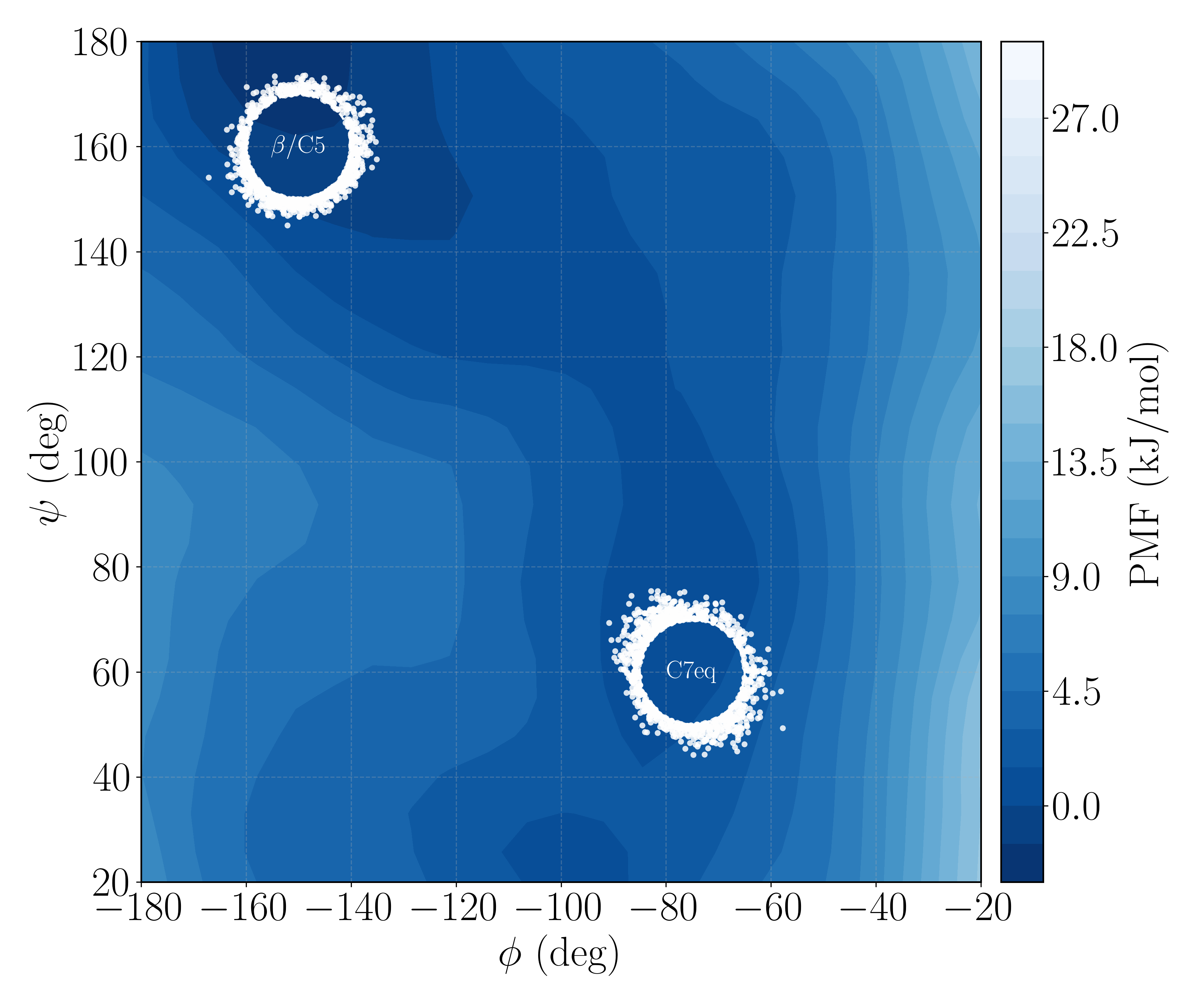
The rates of protein conformational changes control biological function, yet they are among the hardest quantities to compute. The transitions that matter (a loop reorganizing, a dihedral flipping, a domain rotating) are rare on the timescale of the fastest molecular motions, so a direct molecular dynamics trajectory spends essentially all of its steps inside a metastable region and almost none crossing between regions. Waiting for enough spontaneous crossings to estimate a rate can require billions of steps, and the cost grows exponentially with the barrier height.
The standard way out is to stop waiting. We decompose a long trajectory into short paths $\Gamma = \{\mathbf{x}_1, \ldots, \mathbf{x}_N\}$, each initiated when the trajectory leaves region A and terminated when it enters region A or B. Paths ending in A are failure paths; those ending in B are success paths. With $\mathcal{K}_\tau(\mathbf{y}\,|\,\mathbf{x})$ the stopped transition kernel at lag $\tau$, the density of a success path factorizes,
Path density
$$ p(\Gamma_{\rm AB}) = \rho_{\rm A}(\mathbf{x}_1) \prod_{i=1}^{N-1} \mathcal{K}_\tau(\mathbf{x}_{i+1}\,|\,\mathbf{x}_i), $$
and the reactive probability is the integral over all success paths, $P_{\rm AB} = \int p(\Gamma)\, d\Gamma$. The rate then follows from the Hill relation (Hill, 2012; Baudel et al., 2023):
Hill relation
$$ r_{\rm AB} = \Phi_{\rm A}\, P_{\rm AB}, \qquad \mathrm{MFPT}_{\rm AB} = 1 / r_{\rm AB}, $$
where $\Phi_{\rm A}$ is the flux of trajectories escaping region A (the inverse mean time between successive first exits). The flux is cheap, because escapes from a region are not rare. All of the difficulty is concentrated in $P_{\rm AB}$: the probability that an escaped trajectory commits to the far region rather than falling back.
2Importance sampling and the path weight
For a genuine rare event the success probability is tiny compared with that of a failure path, so we modify the transition kernel with an importance function $I(\mathbf{x})$ (Cai et al., 2002; de Koning et al., 2005) that biases the walker toward B:
Biased kernel
$$ \mathcal{K}'_\tau(\mathbf{y}\,|\,\mathbf{x}) = Z_\tau^{-1}(\mathbf{x})\, \frac{I(\mathbf{y})}{I(\mathbf{x})}\, \mathcal{K}_\tau(\mathbf{y}\,|\,\mathbf{x}), \qquad Z_\tau(\mathbf{x}) = \int_\Omega d\mathbf{y}\, \frac{I(\mathbf{y})}{I(\mathbf{x})}\, \mathcal{K}_\tau(\mathbf{y}\,|\,\mathbf{x}), $$
where the normalization factor $Z_\tau(\mathbf{x})$, computed on the fly by Monte Carlo integration, keeps $\mathcal{K}'_\tau$ a probability density. Propagating a walker under $\mathcal{K}'_\tau$ and reweighting back to the true dynamics attaches to each path a correction factor built from those same normalizations, and this defines the path weight:
Path weight
$$ p'(\Gamma_{\rm AB}) = \frac{I(\mathbf{x}_N)}{I(\mathbf{x}_1)} \left[\prod_{i=1}^{N-1} Z_\tau^{-1}(\mathbf{x}_i)\right] p(\Gamma_{\rm AB}), \qquad W(\Gamma) := \prod_{i=1}^{N-1} Z_\tau(\mathbf{x}_i). $$
Setting $I(\mathbf{x}) = 0$ on A and $I(\mathbf{x}) = 1$ on B, the optimality condition $\int I(\mathbf{y})\, \mathcal{K}_\tau(\mathbf{y}\,|\,\mathbf{x})\, d\mathbf{y} = I(\mathbf{x})$ is exactly the backward equation whose solution is the committor. When $I$ equals this optimal importance function every $Z_\tau = 1$, and the bias enhances success paths by the known factor $I(\mathbf{x}_N)/I(\mathbf{x}_1)$. When $I$ is imperfect, the weights $W(\Gamma)$ restore the unbiased statistics exactly. The reweighted estimator of the reactive probability is
Reweighted estimator
$$ \widehat{P}_{\rm AB} = \frac{1}{N_p} \sum_{i=1}^{N_p} I(\mathbf{x}_1^{(i)})\, W(\Gamma_i)\, \mathbf{1}\!\left[\Gamma_i \in \{\Gamma_{\rm AB}\}\right], $$
which is unbiased for any importance function, including an imperfect learned committor. This is the crucial licence the method operates under: errors in the guide degrade efficiency, not correctness. A neural network that is merely a decent approximation of the committor still yields a statistically exact rate, provided we can afford the variance it induces.
3The weight-variance problem
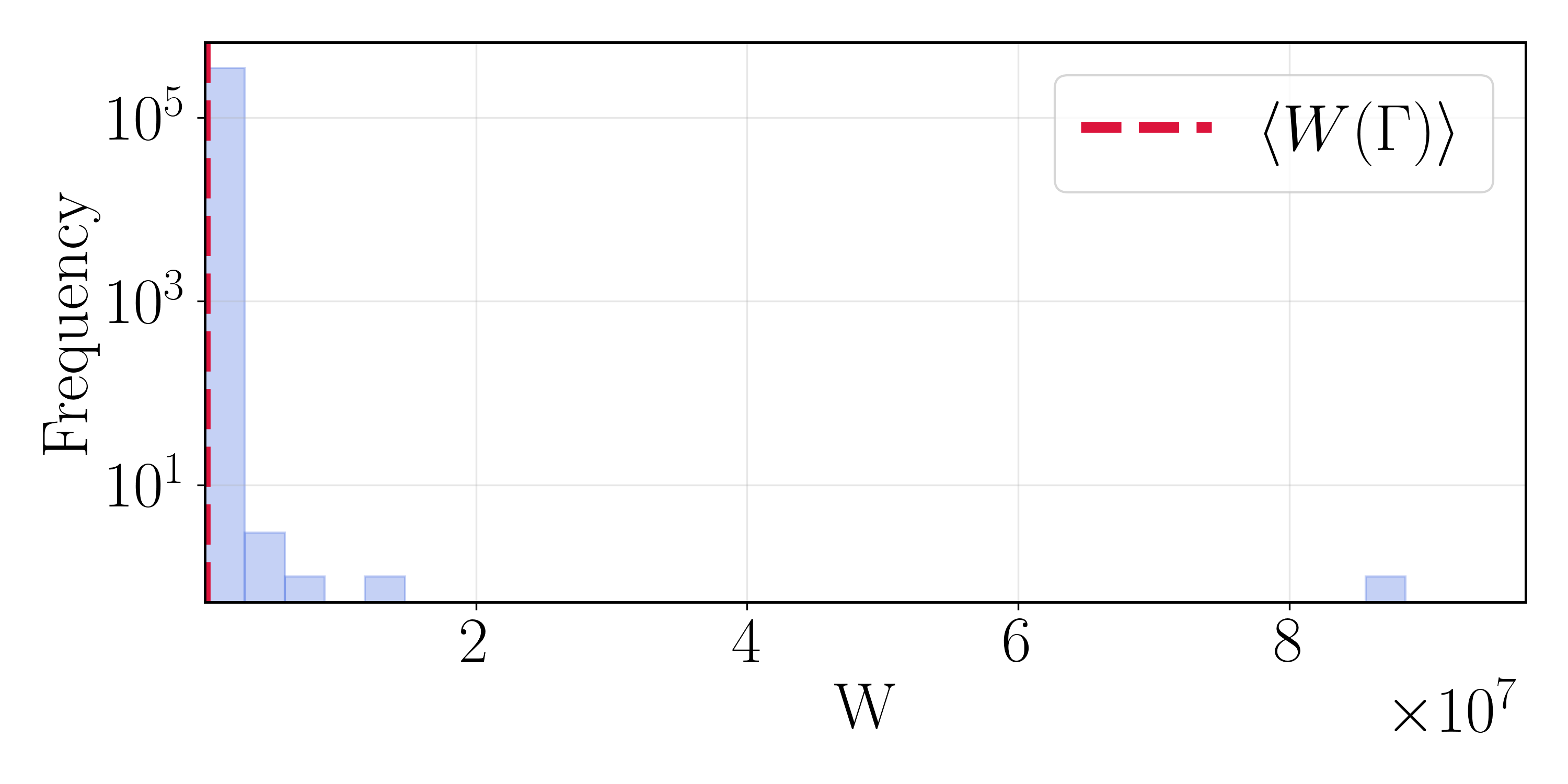
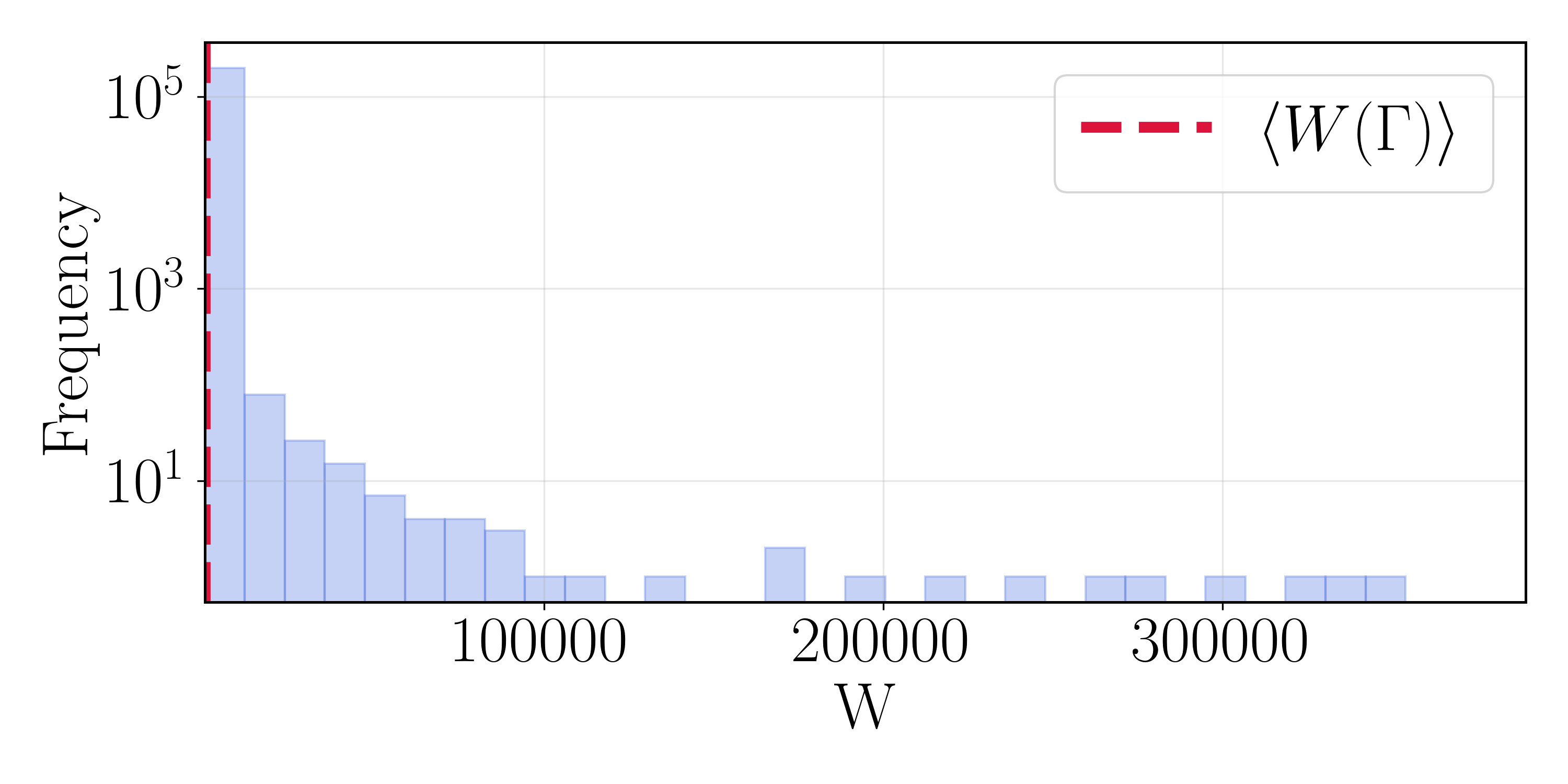
Unbiasedness is not enough. Because $W(\Gamma)$ is a product of $N-1$ fluctuating factors, its variance grows exponentially in path length,
Variance growth
$$ \mathrm{Var}[W] \sim e^{cN}, \qquad c > 0, $$
the classic weight-degeneracy pathology of sequential importance sampling. The efficiency of the estimator is governed by the effective sample size,
Effective sample size
$$ \mathrm{ESS} = \frac{\left(\sum_i W_i\right)^2}{\sum_i W_i^2}, $$
which collapses from $N_p$ toward $1$ as a single weight comes to dominate. Proteins are close to the worst case for this pathology. The fast, stiff vibrational modes (bond stretches, angle bends) make the per-step factors $Z_\tau(\mathbf{x}_i)$ noisy at every step without advancing the slow $(\phi,\psi)$ reorganization we actually care about. Weight noise accumulates on the fast clock while progress accumulates on the slow one. Degeneracy therefore sets in quickly, and a raw importance-sampled estimator is unusable in practice.